Using Activation Functions in Neural Networks

 Activation functions play an integral role in neural networks by introducing nonlinearity. This nonlinearity allows neural networks to develop complex representations and functions based on the inputs that would not be possible with a simple linear regression model.

Many different nonlinear activation functions have been proposed throughout the history of neural networks. In this post, you will explore three popular ones: sigmoid, tanh, and ReLU.

After reading this article, you will learn:

• Why nonlinearity is important in a neural network
• How different activation functions can contribute to the vanishing gradient problem
• Sigmoid, tanh, and ReLU activation functions
• How to use different activation functions in your TensorFlow model

Let’s get started.

Overview

This article is split into five sections; they are:

• Why do we need nonlinear activation functions
• Sigmoid function and vanishing gradient
• Hyperbolic tangent function
• Rectified Linear Unit (ReLU)
• Using the activation functions in practice

Why Do We Need Nonlinear Activation Functions

You might be wondering, why all this hype about nonlinear activation functions? Or why can’t we just use an identity function after the weighted linear combination of activations from the previous layer? Using multiple linear layers is basically the same as using a single linear layer. This can be seen through a simple example.

Let’s say you have a one hidden layer neural network, each with two hidden neurons.

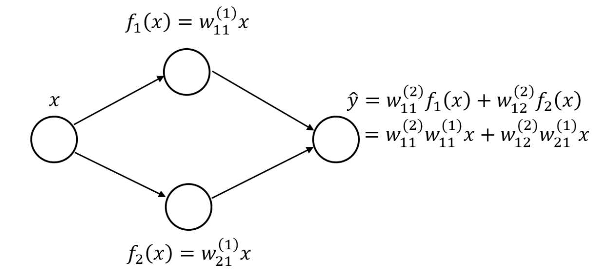
Single hidden layer neural network with linear layers

You can then rewrite the output layer as a linear combination of the original input variable if you used a linear hidden layer. If you had more neurons and weights, the equation would be a lot longer with more nesting and more multiplications between successive layer weights. However, the idea remains the same: You can represent the entire network as a single linear layer.

To make the network represent more complex functions, you would need nonlinear activation functions. Let’s start with a popular example, the sigmoid function.

Sigmoid Function and Vanishing Gradient

The sigmoid activation function is a popular choice for the nonlinear activation function for neural networks. One reason it’s popular is that it has output values between 0 and 1, which mimic probability values. Hence it is used to convert the real-valued output of a linear layer to a probability, which can be used as a probability output. This also makes it an important part of logistic regression methods, which can be used directly for binary classification.

The sigmoid function is commonly represented by $�$ and has the form $�=\frac{1}{1+{�}^{-1}}$. In TensorFlow, you can call the sigmoid function from the Keras library as follows:

1 2 3 4 5

import tensorflow as tf from tensorflow.keras.activations import sigmoid   input_array = tf.constant([-1, 0, 1], dtype=tf.float32) print (sigmoid(input_array))

This gives the following output:

1	tf.Tensor([0.26894143 0.5        0.7310586 ], shape=(3,), dtype=float32)

You can also plot the sigmoid function as a function of $�$,

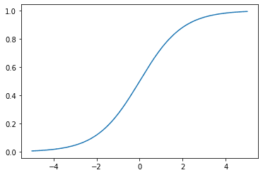
Sigmoid activation function

When looking at the activation function for the neurons in a neural network, you should also be interested in its derivative due to backpropagation and the chain rule, which would affect how the neural network learns from data.

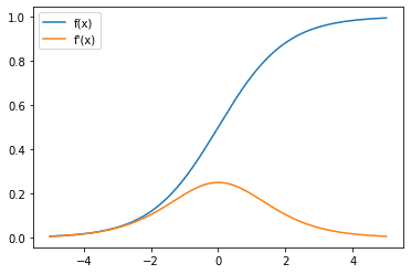
Sigmoid activation function (blue) and gradient (orange)

Here, you can observe that the gradient of the sigmoid function is always between 0 and 0.25. And as the $�$ tends to positive or negative infinity, the gradient tends to zero. This could contribute to the vanishing gradient problem, meaning when the inputs are at some large magnitude of $�$ (e.g., due to the output from earlier layers), the gradient is too small to initiate the correction.

Vanishing gradient is a problem because the chain rule is used in backpropagation in deep neural networks. Recall that in neural networks, the gradient (of the loss function) at each layer is the gradient at its subsequent layer multiplied by the gradient of its activation function. As there are many layers in the network, if the gradient of the activation functions is less than 1, the gradient at some layer far away from the output will be close to zero. And any layer with a gradient close to zero will stop the gradient propagation further back to the earlier layers.

Since the sigmoid function is always less than 1, a network with more layers would exacerbate the vanishing gradient problem. Furthermore, there is a saturation region where the gradient of the sigmoid tends to 0, which is where the magnitude of $�$ is large. So, if the output of the weighted sum of activations from previous layers is large, then you would have a very small gradient propagating through this neuron as the derivative of the activation $�$ with respect to the input to the activation function would be small (in the saturation region).

Granted, there is also the derivative of the linear term with respect to the previous layer’s activations which might be greater than 1 for the layer since the weight might be large, and it’s a sum of derivatives from the different neurons. However, it might still raise concern at the start of training as weights are usually initialized to be small.

Hyperbolic Tangent Function

Another activation function to consider is the tanh activation function, also known as the hyperbolic tangent function. It has a larger range of output values compared to the sigmoid function and a larger maximum gradient. The tanh function is a hyperbolic analog to the normal tangent function for circles that most people are familiar with.

Plotting out the tanh function:

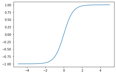
Tanh activation function

Let’s look at the gradient as well:

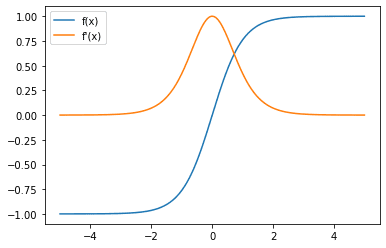
Tanh activation function (blue) and gradient (orange)

Notice that the gradient now has a maximum value of 1, compared to the sigmoid function, where the largest gradient value is 0. This makes a network with tanh activation less susceptible to the vanishing gradient problem. However, the tanh function also has a saturation region, where the value of the gradient tends toward as the magnitude of the input $�$ gets larger.

In TensorFlow, you can implement the tanh activation on a tensor using the tanh function in Keras’s activations module:

1 2 3 4 5

import tensorflow as tf from tensorflow.keras.activations import tanh   input_array = tf.constant([-1, 0, 1], dtype=tf.float32) print (tanh(input_array))

This gives the output:

1	tf.Tensor([-0.7615942  0.         0.7615942], shape=(3,), dtype=float32)

Rectified Linear Unit (ReLU)

The last activation function to cover in detail is the Rectified Linear Unit, also popularly known as ReLU. It has become popular recently due to its relatively simple computation. This helps to speed up neural networks and seems to get empirically good performance, which makes it a good starting choice for the activation function.

The ReLU function is a simple $max(0,�)$ function, which can also be thought of as a piecewise function with all inputs less than 0 mapping to 0 and all inputs greater than or equal to 0 mapping back to themselves (i.e., identity function). Graphically,

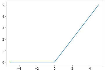
ReLU activation function

Next up, you can also look at the gradient of the ReLU function:

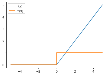
ReLU activation function (blue line) and gradient (orange)

Notice that the gradient of ReLU is 1 whenever the input is positive, which helps address the vanishing gradient problem. However, whenever the input is negative, the gradient is 0. This can cause another problem, the dead neuron/dying ReLU problem, which is an issue if a neuron is persistently inactivated.

In this case, the neuron can never learn, and its weights are never updated due to the chain rule as it has a 0 gradient as one of its terms. If this happens for all data in your dataset, then it can be very difficult for this neuron to learn from your dataset unless the activations in the previous layer change such that the neuron is no longer “dead.”

To use the ReLU activation in TensorFlow:

1 2 3 4 5

import tensorflow as tf from tensorflow.keras.activations import relu   input_array = tf.constant([-1, 0, 1], dtype=tf.float32) print (relu(input_array))

This gives the following output:

1	tf.Tensor([0. 0. 1.], shape=(3,), dtype=float32)

The three activation functions reviewed above show that they are all monotonically increasing functions. This is required; otherwise, you cannot apply the gradient descent algorithm.

Now that you’ve explored some common activation functions and how to use them in TensorFlow. Let’s take a look at how you can use these in practice in an actual model.

Using Activation Functions in Practice

Before exploring the use of activation functions in practice, let’s look at another common way to use activation functions when combining them with another Keras layer. Let’s say you want to add a ReLU activation on top of a Dense layer. One way you can do this following the above methods shown is to do:

1 2	x = Dense(units=10)(input_layer) x = relu(x)

However, for many Keras layers, you can also use a more compact representation to add the activation on top of the layer:

1	x = Dense(units=10, activation=”relu”)(input_layer)

Using this more compact representation, let’s build our LeNet5 model using Keras:

1 2 3 4 5 6 7 8 9 10 11 12 13 14 15 16 17 18 19 20 21 22 23 24

import tensorflow as tf import tensorflow.keras as keras from tensorflow.keras.layers import Dense, Input, Flatten, Conv2D, BatchNormalization, MaxPool2D from tensorflow.keras.models import Model   (trainX, trainY), (testX, testY) = keras.datasets.cifar10.load_data()   input_layer = Input(shape=(32,32,3,)) x = Conv2D(filters=6, kernel_size=(5,5), padding="same", activation="relu")(input_layer) x = MaxPool2D(pool_size=(2,2))(x) x = Conv2D(filters=16, kernel_size=(5,5), padding="same", activation="relu")(x) x = MaxPool2D(pool_size=(2, 2))(x) x = Conv2D(filters=120, kernel_size=(5,5), padding="same", activation="relu")(x) x = Flatten()(x) x = Dense(units=84, activation="relu")(x) x = Dense(units=10, activation="softmax")(x)   model = Model(inputs=input_layer, outputs=x)   print(model.summary())   model.compile(optimizer="adam", loss=tf.keras.losses.SparseCategoricalCrossentropy(), metrics="acc")   history = model.fit(x=trainX, y=trainY, batch_size=256, epochs=10, validation_data=(testX, testY))

And running this code gives the following output:

1 2 3 4 5 6 7 8 9 10 11 12 13 14 15 16 17 18 19 20 21 22 23 24 25 26 27 28 29 30 31 32 33 34 35 36 37 38 39 40 41 42 43 44 45 46 47 48 49 50

Model: "model" _________________________________________________________________ Layer (type)                Output Shape              Param #   ================================================================= input_1 (InputLayer)        [(None, 32, 32, 3)]       0                                                                          conv2d (Conv2D)             (None, 32, 32, 6)         456                                                                        max_pooling2d (MaxPooling2D  (None, 16, 16, 6)        0         )                                                                                                                                conv2d_1 (Conv2D)           (None, 16, 16, 16)        2416                                                                        max_pooling2d_1 (MaxPooling  (None, 8, 8, 16)         0         2D)                                                                                                                              conv2d_2 (Conv2D)           (None, 8, 8, 120)         48120                                                                      flatten (Flatten)           (None, 7680)              0                                                                          dense (Dense)               (None, 84)                645204                                                                      dense_1 (Dense)             (None, 10)                850                                                                        ================================================================= Total params: 697,046 Trainable params: 697,046 Non-trainable params: 0 _________________________________________________________________ None Epoch 1/10 196/196 [==============================] - 14s 11ms/step - loss: 2.9758 acc: 0.3390 - val_loss: 1.5530 - val_acc: 0.4513 Epoch 2/10 196/196 [==============================] - 2s 8ms/step - loss: 1.4319 - acc: 0.4927 - val_loss: 1.3814 - val_acc: 0.5106 Epoch 3/10 196/196 [==============================] - 2s 8ms/step - loss: 1.2505 - acc: 0.5583 - val_loss: 1.3595 - val_acc: 0.5170 Epoch 4/10 196/196 [==============================] - 2s 8ms/step - loss: 1.1127 - acc: 0.6094 - val_loss: 1.2892 - val_acc: 0.5534 Epoch 5/10 196/196 [==============================] - 2s 8ms/step - loss: 0.9763 - acc: 0.6594 - val_loss: 1.3228 - val_acc: 0.5513 Epoch 6/10 196/196 [==============================] - 2s 8ms/step - loss: 0.8510 - acc: 0.7017 - val_loss: 1.3953 - val_acc: 0.5494 Epoch 7/10 196/196 [==============================] - 2s 8ms/step - loss: 0.7361 - acc: 0.7426 - val_loss: 1.4123 - val_acc: 0.5488 Epoch 8/10 196/196 [==============================] - 2s 8ms/step - loss: 0.6060 - acc: 0.7894 - val_loss: 1.5356 - val_acc: 0.5435 Epoch 9/10 196/196 [==============================] - 2s 8ms/step - loss: 0.5020 - acc: 0.8265 - val_loss: 1.7801 - val_acc: 0.5333 Epoch 10/10 196/196 [==============================] - 2s 8ms/step - loss: 0.4013 - acc: 0.8605 - val_loss: 1.8308 - val_acc: 0.5417

And that’s how you can use different activation functions in your TensorFlow models!

Further Reading

Other examples of activation functions:

• Leaky ReLU (ReLU where the negative has a non-zero gradient): https://www.tensorflow.org/api_docs/python/tf/keras/layers/LeakyReLU 
• Parametric ReLU (non-zero gradient on negative is a learned parameter): https://arxiv.org/abs/1502.01852
• Maxout unit: https://arxiv.org/abs/1302.4389

Summary

In this post, you have seen why activation functions are important to allow for the complex neural networks that are common in deep learning today. You have also seen some popular activation functions, their derivatives, and how to integrate them into your TensorFlow models.

Specifically, you learned:

• Why nonlinearity is important in a neural network
• How different activation functions can contribute to the vanishing gradient problem
• Sigmoid, tanh, and ReLU activation functions
• How to use different activation functions in your TensorFlow model