A Gentle Introduction to Bayesian Regression

 

A Gentle Introduction to Bayesian Regression
Image by Editor | ChatGPT

In this article, you will learn:

• The fundamental difference between traditional regression, which uses single fixed values for its parameters, and Bayesian regression, which models them as probability distributions.
• How this probabilistic approach allows the model to produce a full distribution of possible outcomes, thereby quantifying the uncertainty in its predictions.
• How to implement a simple Bayesian regression model in Python with scikit-learn.

Introduction

In machine learning, regression models are a widely used family of models for making predictions on numeric, continuous variables, such as house prices, temperatures, or stock values. Traditional regression models are defined by precise parameters or weights and typically assume no uncertainty in these estimates. Bayesian regression was introduced to model the relationship between predictor and target variables probabilistically, introducing uncertainty into the modeling process.

Traditional Regression Models

Traditional regression models produce predictions on target continuous variables, for instance, house prices, in the form of an estimate, ˆ𝑦, that is a single, crisp value, e.g., the estimated price of a house whose attributes have been passed to the model as inputs. For instance, the equation of a linear regression model with n input variables (e.g. house attributes) is given by the following linear equation:

ˆ𝑦 =𝛽0 +𝛽1⁢𝑥1 +𝛽2⁢𝑥2 +… +𝛽𝑛⁢𝑥𝑛 +𝜖

where 𝜖 is the error term, and 𝛽0,…,𝛽𝑛 are the weights associated with the input variables, plus a bias term, 𝛽0. A real-world instantiation of this equation to a specific learned model to predict house prices could look like this:

ˆ𝑦 =50000 +150 ⋅𝑥1 +10000 ⋅𝑥2–2000 ⋅𝑥3 +𝜖

where:

• 𝑥1 is the house’s square footage in square meters.
• 𝑥2 is the number of bedrooms.
• 𝑥3 is the age of the house in years — notice the minus sign for the weight accompanying this feature, which means older houses contribute to lower price predictions. This makes sense, as older houses tend to be cheaper.

The 50000, 150, 10000, and -2000 values in the above model are its parameter values or weights. This is an important point to remember as we continue.

How Does Bayesian Regression Work?

So, what makes Bayesian regression different from this? Unlike traditional regression, which returns a single value as the predicted estimate and similarly has weights learned as precise values, a Bayesian regression model deals with probability distributions over the possible parameter values, thereby accounting for uncertainty in predictions. Put another way, in a Bayesian regression model, each weight 𝛽𝑖 becomes a random variable with its associated probability distribution.

The learning process is adapted accordingly: instead of seeking a single “best-fitting” set of n+1 weights, 𝛽0,𝛽1,𝛽2,…,𝛽𝑛, we try to find a posterior distribution over parameters, given the training data (a set of instances with a known output or target value).

Importantly, since weights are modeled as distributions, the resulting predictions, ˆ𝑦, also become distributions rather than crisp, single-point estimates. Therefore, the prediction becomes uncertain.

Why would we be interested in predictions that are uncertain rather than precise?

Bayesian regression makes sense in scenarios where understanding and accounting for uncertainty is as important as making the prediction itself. For instance, in high-stakes scenarios like medical diagnosis, we may want to know not only what the model’s prediction is but also how confident or uncertain the model is about that prediction. In cases where confidence is lower, a health professional can use their professional judgment to interpret the results. Other scenarios where Bayesian regression adds practical value are autonomous vehicles and financial forecasting: in these cases, making decisions upon potentially wrong precise predictions could have a significant cost or yield dangerous outcomes; hence, having predictions modeled as probability distributions is a more informative approach to balance possible risks or seek additional information if necessary.

Bayesian Regression: A Simple Example

Let’s show a very simple example to understand how Bayesian regression works.

Assume we would like to estimate the price of a house based only on one attribute: its square footage. The input attribute is denoted by 𝑥1. A classical regression model for this problem would look something like this:

ˆ𝑦 =50000 +150 ⋅𝑥1

In Bayesian regression, the two model weights, 𝛽0 and 𝛽1, do not take precise values like 50000 and 150, respectively, but are instead learned as probability distributions. For example:

• The bias term (also called intercept) 𝛽0 follows a normal distribution, that is:

  𝛽0 ∼𝑁⁡(50000,50002)

• Meanwhile, the slope or weight accompanying the single input feature, 𝛽1, also becomes a normal distribution, namely:

  𝛽1 ∼𝑁⁡(150,202)

Recall that the two arguments defining a normal distribution are its mean and variance.

How is the house price predicted then? Instead of returning a single price prediction, the model applies inference by sampling from these two distributions associated with weights, thereby producing a range of possible predictions. For example, for a 100-square-meter house, this is what two samples might look like:

1. Sample 1: 𝛽0 =52000, 𝛽1 =160, with price ˆ𝑦 =52000 +160 ⋅100 =68,000 USD
2. Sample 2: 𝛽0 =49000, 𝛽1 =140, with price ˆ𝑦 =49000 +140 ⋅100 =63,000 USD

By sampling a large number of times, we end up obtaining a distribution of predicted prices, in which certain ranges of prices will appear more frequently than others and, therefore, have a higher probability than others. Based on this, we could end up formulating predictions as confidence intervals, like:

The predicted value of this house is approximately 65,500 USD, with a 95% confidence interval between 61,000 USD and 70,000 USD.

As discussed earlier, in some real-world use cases, these uncertain predictions are more valuable and helpful in effective and informed decision-making.

Bayesian Regression in Python with Scikit-learn

Fortunately, implementing Bayesian regression in Python is straightforward with scikit-learn. The linear_model module provides a BayesianRidge object that can be used to perform Bayesian regression. This object works similarly to other scikit-learn models: you create an instance of the model, fit it to your training data, and then use it to make predictions. A key difference, however, is that when you call the predict method, you can also request the standard deviation of the predictions, which gives you a measure of the model’s uncertainty.

Here is a simple code example that demonstrates how to use BayesianRidge to fit a model to some sample data and then make a prediction, including the uncertainty.

import numpy as np from sklearn.linear_model import BayesianRidge   np.random.seed(42)   # Sample data (house square footage) with added noise to demonstrate uncertainty X = np.array([[50], [100], [150], [200], [250]])   # Target values (house prices) with added random noise y = (np.array([100000, 200000, 300000, 400000, 500000]) + np.random.normal(0, 30000, X.shape[0]))   # Create and fit the model with adjusted parameters to emphasize uncertainty # alpha_1, alpha_2, lambda_1, lambda_2 control the prior distributions over precision of weights and noise model = BayesianRidge(alpha_1=1e-6, alpha_2=1e-6, lambda_1=1e-6, lambda_2=1e-6) model.fit(X, y)   # Predict the price and uncertainty for a new 120 m^2 house new_house_sqft = np.array([[120]]) mean_prediction, std_prediction = model.predict(new_house_sqft, return_std=True)   print(f"Predicted price for 120 m^2: ${mean_prediction[0]:,.2f}") print(f"Uncertainty (std dev) for 120 m^2: ${std_prediction[0]:,.2f}")   # Predict for an extrapolated value to show increased uncertainty (350 m^2) extrapolated_sqft = np.array([[350]]) mean_extrapolated, std_extrapolated = model.predict(extrapolated_sqft, return_std=True) print(f"Predicted price for 350 m^2 (extrapolated): ${mean_extrapolated[0]:,.2f}") print(f"Uncertainty (std dev) for 350 m^2: ${std_extrapolated[0]:,.2f}")

Output:

Predicted price for 120 m^2: $253,679.60 Uncertainty (std dev) for 120 m^2: $26,625.02 Predicted price for 350 m^2 (extrapolated): $714,373.37 Uncertainty (std dev) for 350 m^2: $51,462.04

In the above code:

• alpha_1: Sets our initial assumption for how simple or complex the relationship between the inputs and output should be by influencing the model’s weights
• alpha_2: Works with alpha_1 to control how strongly the model holds on to its initial assumption about the relationship’s simplicity versus learning from the data.
• lambda_1: Sets our initial assumption about how much “noise” or random error is present in the data we are training on.
• lambda_2: Works with lambda_1 to control how strongly the model holds on to its initial assumption about the noise level.

The following visualization shows the noise in the training data, the best-fit line, and most importantly, how the uncertainty band widens as we move away from the training data points, especially when extrapolating. This visually demonstrates the core advantage of Bayesian regression: its ability to quantify predictive uncertainty.

import matplotlib.pyplot as plt   # Generate a wider range of square footage values for plotting, including extrapolation X_plot = np.linspace(0, 400, 200).reshape(-1, 1)   # Get the mean and standard deviation of the predictions for the plot y_mean, y_std = model.predict(X_plot, return_std=True)   # Plot the results plt.figure(figsize=(10, 6))   # Plot the original noisy data points plt.scatter(X, y, color='blue', label='Training Data (with noise)')   # Plot the regression line plt.plot(X_plot, y_mean, color='red', label='Bayesian Ridge Mean Prediction')   # Plot the uncertainty area (1 standard deviation) plt.fill_between(X_plot.ravel(), y_mean - y_std, y_mean + y_std, color='pink', alpha=0.5, label='Uncertainty (1 std dev)')   # Plot the 95% confidence interval (approx. 2 std dev) for richer illustration plt.fill_between(X_plot.ravel(), y_mean - 2 * y_std, y_mean + 2 * y_std, color='lightcoral', alpha=0.2, label='Uncertainty (2 std dev / 95% CI)')   # Visualization labels and presentation plt.title('Bayesian Regression with Quantified Uncertainty') plt.xlabel('Square Footage') plt.ylabel('House Price') plt.legend() plt.grid(True) plt.show()

And our generated visualization:

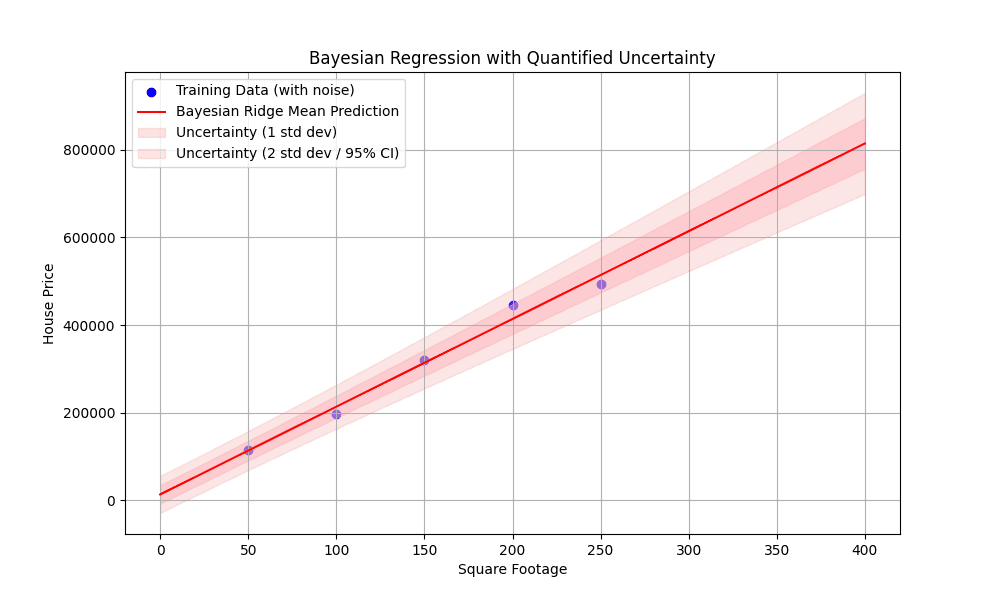
Figure 1: Bayesian regression with quantified uncertainty

Final Thoughts

Bayesian regression can be viewed as the uncertain and probabilistic counterpart to classical regression models, which are one of the most widespread types of machine learning models for making predictions in many real-world applications. This article has provided a gentle introduction to the basics and usefulness of this regression technique.

Interested in specific Bayesian regression techniques and models? Among the most popular ones, we have Bayesian Linear Regression, Bayesian Ridge Regression, and Gaussian Process Regression (GPR)