Artificial Intelligence , Machine Learning and Data Science Hubspot

Unlock the Power of Artificial Intelligence, Machine Learning, and Data Science with our Blog Discover the latest insights, trends, and innovations in Artificial Intelligence (AI), Machine Learning (ML), and Data Science through our informative and engaging Hubspot blog. Gain a deep understanding of how these transformative technologies are shaping industries and revolutionizing the way we work. Stay updated with cutting-edge advancements, practical applications, and real-world use.

Monday, 19 February 2024

Application of differentiations in neural networks

Differential calculus is an important tool in machine learning algorithms. Neural networks in particular, the gradient descent algorithm depends on the gradient, which is a quantity computed by differentiation.

In this tutorial, we will see how the back-propagation technique is used in finding the gradients in neural networks.

After completing this tutorial, you will know

What is a total differential and total derivative
How to compute the total derivatives in neural networks
How back-propagation helped in computing the total derivatives

Let’s get started

Application of differentiations in neural networks
Photo by Freeman Zhou, some rights reserved.

Tutorial overview

This tutorial is divided into 5 parts; they are:

Total differential and total derivatives
Algebraic representation of a multilayer perceptron model
Finding the gradient by back-propagation
Matrix form of gradient equations
Implementing back-propagation

Total differential and total derivatives

For a function such as $� (�)$ , we call denote its derivative as $�^{'} (�)$ or $\frac{� �}{� �}$ . But for a multivariate function, such as $� (�, �)$ , we have a partial derivative of $�$ with respect to $�$ denoted as $\frac{� �}{� �}$ , or sometimes written as $�_{�}$ . A partial derivative is obtained by differentiation of $�$ with respect to $�$ while assuming the other variable $�$ is a constant. Therefore, we use $�$ instead of $�$ as the symbol for differentiation to signify the difference.

However, what if the $�$ and $�$ in $� (�, �)$ are both function of $�$ ? In other words, we can write $� (�)$ and $� (�)$ and $� (� (�), � (�))$ . So $�$ determines the value of $�$ and $�$ and in turn, determines $� (�, �)$ . In this case, it is perfectly fine to ask what is $\frac{� �}{� �}$ , as $�$ is eventually determined by $�$ .

This is the concept of total derivatives. In fact, for a multivariate function $� (�, �, �) = � (� (�), � (�), � (�))$ , we always have
$\frac{� �}{� �} = \frac{� �}{� �} \frac{� �}{� �} + \frac{� �}{� �} \frac{� �}{� �} + \frac{� �}{� �} \frac{� �}{� �}$
The above notation is called the total derivative because it is sum of the partial derivatives. In essence, it is applying chain rule to find the differentiation.

If we take away the $� �$ part in the above equation, what we get is an approximate change in $�$ with respect to $�$ , i.e.,
$� � = \frac{� �}{� �} � � + \frac{� �}{� �} � � + \frac{� �}{� �} � �$
We call this notation the total differential.

Algebraic representation of a multilayer perceptron model

Consider the network:

An example of neural network. Source: https://commons.wikimedia.org/wiki/File:Multilayer_Neural_Network.png

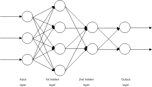
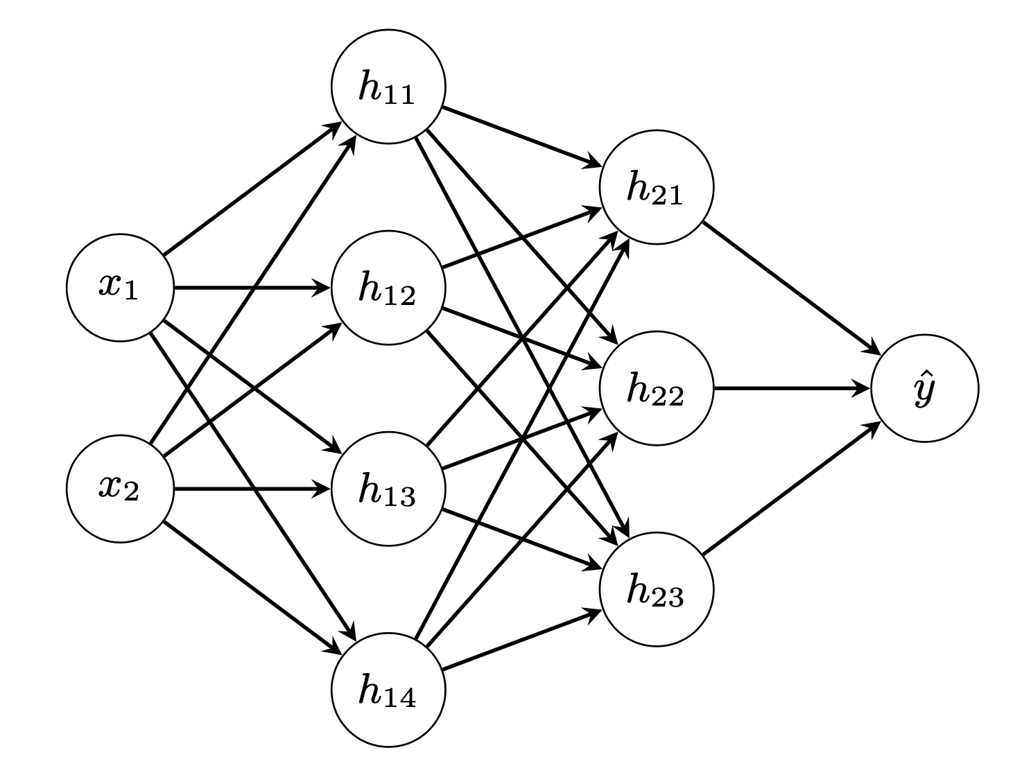
This is a simple, fully-connected, 4-layer neural network. Let’s call the input layer as layer 0, the two hidden layers the layer 1 and 2, and the output layer as layer 3. In this picture, we see that we have $�_{0} = 3$ input units, and $�_{1} = 4$ units in the first hidden layer and $�_{2} = 2$ units in the second input layer. There are $�_{3} = 2$ output units.

If we denote the input to the network as $�_{�}$ where $� = 1, \dots, �_{0}$ and the network’s output as ${\hat{�}}_{�}$ where $� = 1, \dots, �_{3}$ . Then we can write

$\begin{aligned} ℎ_{1 �} & = �_{1} (\sum_{� = 1}^{�_{0}} �_{� �}^{(1)} �_{�} + �_{�}^{(1)}) & for � & = 1, \dots, �_{1} \\ ℎ_{2 �} & = �_{2} (\sum_{� = 1}^{�_{1}} �_{� �}^{(2)} ℎ_{1 �} + �_{�}^{(2)}) & � & = 1, \dots, �_{2} \\ {\hat{�}}_{�} & = �_{3} (\sum_{� = 1}^{�_{2}} �_{� �}^{(3)} ℎ_{2 �} + �_{�}^{(3)}) & � & = 1, \dots, �_{3} \end{aligned}$

Here the activation function at layer $�$ is denoted as $�_{�}$ . The outputs of first hidden layer are denoted as $ℎ_{1 �}$ for the $�$ -th unit. Similarly, the outputs of second hidden layer are denoted as $ℎ_{2 �}$ . The weights and bias of unit $�$ in layer $�$ are denoted as $�_{� �}^{(�)}$ and $�_{�}^{(�)}$ respectively.

In the above, we can see that the output of layer $� - 1$ will feed into layer $�$ . Therefore, while ${\hat{�}}_{�}$ is expressed as a function of $ℎ_{2 �}$ , but $ℎ_{2 �}$ is also a function of $ℎ_{1 �}$ and in turn, a function of $�_{�}$ .

The above describes the construction of a neural network in terms of algebraic equations. Training a neural network would need to specify a *loss function* as well so we can minimize it in the training loop. Depends on the application, we commonly use cross entropy for categorization problems or mean squared error for regression problems. With the target variables as $�_{�}$ , the mean square error loss function is specified as
$� = \sum_{� = 1}^{�_{3}} (�_{�} - {\hat{�}}_{�})^{2}$

Want to Get Started With Calculus for Machine Learning?

Take my free 7-day email crash course now (with sample code).

Click to sign-up and also get a free PDF Ebook version of the course.

Finding the gradient by back-propagation

In the above construct, $�_{�}$ and $�_{�}$ are from the dataset. The parameters to the neural network are $�$ and $�$ . While the activation functions $�_{�}$ are by design the outputs at each layer $ℎ_{1 �}$ , $ℎ_{2 �}$ , and ${\hat{�}}_{�}$ are dependent variables. In training the neural network, our goal is to update $�$ and $�$ in each iteration, namely, by the gradient descent update rule:
$\begin{aligned} �_{� �}^{(�)} & = �_{� �}^{(�)} - � \frac{� �}{� �_{� �}^{(�)}} \\ �_{�}^{(�)} & = �_{�}^{(�)} - � \frac{� �}{� �_{�}^{(�)}} \end{aligned}$
where $�$ is the learning rate parameter to gradient descent.

From the equation of $�$ we know that $�$ is not dependent on $�_{� �}^{(�)}$ or $�_{�}^{(�)}$ but on ${\hat{�}}_{�}$ . However, ${\hat{�}}_{�}$ can be written as function of $�_{� �}^{(�)}$ or $�_{�}^{(�)}$ eventually. Let’s see one by one how the weights and bias at layer $�$ can be connected to ${\hat{�}}_{�}$ at the output layer.

We begin with the loss metric. If we consider the loss of a single data point, we have
$\begin{aligned} � & = \sum_{� = 1}^{�_{3}} (�_{�} - {\hat{�}}_{�})^{2} \\ \frac{� �}{� {\hat{�}}_{�}} & = 2 (�_{�} - {\hat{�}}_{�}) & for � & = 1, \dots, �_{3} \end{aligned}$
Here we see that the loss function depends on all outputs ${\hat{�}}_{�}$ and therefore we can find a partial derivative $\frac{� �}{� {\hat{�}}_{�}}$ .

Now let’s look at the output layer:
$\begin{aligned} {\hat{�}}_{�} & = �_{3} (\sum_{� = 1}^{�_{2}} �_{� �}^{(3)} ℎ_{2 �} + �_{�}^{(3)}) & for � & = 1, \dots, �_{3} \\ \frac{� �}{� �_{� �}^{(3)}} & = \frac{� �}{� {\hat{�}}_{�}} \frac{� {\hat{�}}_{�}}{� �_{� �}^{(3)}} & � & = 1, \dots, �_{3}; � = 1, \dots, �_{2} \\ = \frac{� �}{� {\hat{�}}_{�}} �_{3}^{'} (\sum_{� = 1}^{�_{2}} �_{� �}^{(3)} ℎ_{2 �} + �_{�}^{(3)}) ℎ_{2 �} \\ \frac{� �}{� �_{�}^{(3)}} & = \frac{� �}{� {\hat{�}}_{�}} \frac{� {\hat{�}}_{�}}{� �_{�}^{(3)}} & � & = 1, \dots, �_{3} \\ = \frac{� �}{� {\hat{�}}_{�}} �_{3}^{'} (\sum_{� = 1}^{�_{2}} �_{� �}^{(3)} ℎ_{2 �} + �_{�}^{(3)}) \end{aligned}$
Because the weight $�_{� �}^{(3)}$ at layer 3 applies to input $ℎ_{2 �}$ and affects output ${\hat{�}}_{�}$ only. Hence we can write the derivative $\frac{� �}{� �_{� �}^{(3)}}$ as the product of two derivatives $\frac{� �}{� {\hat{�}}_{�}} \frac{� {\hat{�}}_{�}}{� �_{� �}^{(3)}}$ . Similar case for the bias $�_{�}^{(3)}$ as well. In the above, we make use of $\frac{� �}{� {\hat{�}}_{�}}$ , which we already derived previously.

But in fact, we can also write the partial derivative of $�$ with respect to output of second layer $ℎ_{2 �}$ . It is not used for the update of weights and bias on layer 3 but we will see its importance later:
$\begin{aligned} \frac{� �}{� ℎ_{2 �}} & = \sum_{� = 1}^{�_{3}} \frac{� �}{� {\hat{�}}_{�}} \frac{� {\hat{�}}_{�}}{� ℎ_{2 �}} & for � & = 1, \dots, �_{2} \\ = \sum_{� = 1}^{�_{3}} \frac{� �}{� {\hat{�}}_{�}} �_{3}^{'} (\sum_{� = 1}^{�_{2}} �_{� �}^{(3)} ℎ_{2 �} + �_{�}^{(3)}) �_{� �}^{(3)} \end{aligned}$
This one is the interesting one and different from the previous partial derivatives. Note that $ℎ_{2 �}$ is an output of layer 2. Each and every output in layer 2 will affect the output ${\hat{�}}_{�}$ in layer 3. Therefore, to find $\frac{� �}{� ℎ_{2 �}}$ we need to add up every output at layer 3. Thus the summation sign in the equation above. And we can consider $\frac{� �}{� ℎ_{2 �}}$ as the total derivative, in which we applied the chain rule $\frac{� �}{� {\hat{�}}_{�}} \frac{� {\hat{�}}_{�}}{� ℎ_{2 �}}$ for every output $�$ and then sum them up.

If we move back to layer 2, we can derive the derivatives similarly:
$\begin{aligned} ℎ_{2 �} & = �_{2} (\sum_{� = 1}^{�_{1}} �_{� �}^{(2)} ℎ_{1 �} + �_{�}^{(2)}) & for � & = 1, \dots, �_{2} \\ \frac{� �}{� �_{� �}^{(2)}} & = \frac{� �}{� ℎ_{2 �}} \frac{� ℎ_{2 �}}{� �_{� �}^{(2)}} & � & = 1, \dots, �_{2}; � = 1, \dots, �_{1} \\ = \frac{� �}{� ℎ_{2 �}} �_{2}^{'} (\sum_{� = 1}^{�_{1}} �_{� �}^{(2)} ℎ_{1 �} + �_{�}^{(2)}) ℎ_{1 �} \\ \frac{� �}{� �_{�}^{(2)}} & = \frac{� �}{� ℎ_{2 �}} \frac{� ℎ_{2 �}}{� �_{�}^{(2)}} & � & = 1, \dots, �_{2} \\ = \frac{� �}{� ℎ_{2 �}} �_{2}^{'} (\sum_{� = 1}^{�_{1}} �_{� �}^{(2)} ℎ_{1 �} + �_{�}^{(2)}) \\ \frac{� �}{� ℎ_{1 �}} & = \sum_{� = 1}^{�_{2}} \frac{� �}{� ℎ_{2 �}} \frac{� ℎ_{2 �}}{� ℎ_{1 �}} & � & = 1, \dots, �_{1} \\ = \sum_{� = 1}^{�_{2}} \frac{� �}{� ℎ_{2 �}} �_{2}^{'} (\sum_{� = 1}^{�_{1}} �_{� �}^{(2)} ℎ_{1 �} + �_{�}^{(2)}) �_{� �}^{(2)} \end{aligned}$

In the equations above, we are reusing $\frac{� �}{� ℎ_{2 �}}$ that we derived earlier. Again, this derivative is computed as a sum of several products from the chain rule. Also similar to the previous, we derived $\frac{� �}{� ℎ_{1 �}}$ as well. It is not used to train $�_{� �}^{(2)}$ nor $�_{�}^{(2)}$ but will be used for the layer prior. So for layer 1, we have

$\begin{aligned} ℎ_{1 �} & = �_{1} (\sum_{� = 1}^{�_{0}} �_{� �}^{(1)} �_{�} + �_{�}^{(1)}) & for � & = 1, \dots, �_{1} \\ \frac{� �}{� �_{� �}^{(1)}} & = \frac{� �}{� ℎ_{1 �}} \frac{� ℎ_{1 �}}{� �_{� �}^{(1)}} & � & = 1, \dots, �_{1}; � = 1, \dots, �_{0} \\ = \frac{� �}{� ℎ_{1 �}} �_{1}^{'} (\sum_{� = 1}^{�_{0}} �_{� �}^{(1)} �_{�} + �_{�}^{(1)}) �_{�} \\ \frac{� �}{� �_{�}^{(1)}} & = \frac{� �}{� ℎ_{1 �}} \frac{� ℎ_{1 �}}{� �_{�}^{(1)}} & � & = 1, \dots, �_{1} \\ = \frac{� �}{� ℎ_{1 �}} �_{1}^{'} (\sum_{� = 1}^{�_{0}} �_{� �}^{(1)} �_{�} + �_{�}^{(1)}) \end{aligned}$

and this completes all the derivatives needed for training of the neural network using gradient descent algorithm.

Recall how we derived the above: We first start from the loss function $�$ and find the derivatives one by one in the reverse order of the layers. We write down the derivatives on layer $�$ and reuse it for the derivatives on layer $� - 1$ . While computing the output ${\hat{�}}_{�}$ from input $�_{�}$ starts from layer 0 forward, computing gradients are in the reversed order. Hence the name “back-propagation”.

Matrix form of gradient equations

While we did not use it above, it is cleaner to write the equations in vectors and matrices. We can rewrite the layers and the outputs as:
$�_{�} = �_{�} (�_{�}) = �_{�} (�_{�} �_{� - 1} + �_{�})$
where $�_{�}$ is a vector of outputs of layer $�$ , and assume $�_{0} = �$ is the input vector and $�_{3} = \hat{�}$ is the output vector. Also denote $�_{�} = �_{�} �_{� - 1} + �_{�}$ for convenience of notation.

Under such notation, we can represent $\frac{� �}{� �_{�}}$ as a vector (so as that of $�_{�}$ and $�_{�}$ ) and $\frac{� �}{� �_{�}}$ as a matrix. And then if $\frac{� �}{� �_{�}}$ is known, we have
$\begin{aligned} \frac{� �}{� �_{�}} & = \frac{� �}{� �_{�}} ⊙ �_{�}^{'} (�_{�}) \\ \frac{� �}{� �_{�}} & = {(\frac{� �}{� �_{�}})}^{⊤} \cdot �_{�} \\ \frac{� �}{� �_{�}} & = \frac{� �}{� �_{�}} \\ \frac{� �}{� �_{� - 1}} & = {(\frac{� �_{�}}{� �_{� - 1}})}^{⊤} \cdot \frac{� �}{� �_{�}} = �_{�}^{⊤} \cdot \frac{� �}{� �_{�}} \end{aligned}$
where $\frac{� �_{�}}{� �_{� - 1}}$ is a Jacobian matrix as both $�_{�}$ and $�_{� - 1}$ are vectors, and this Jacobian matrix happens to be $�_{�}$ .

Implementing back-propagation

We need the matrix form of equations because it will make our code simpler and avoided a lot of loops. Let’s see how we can convert these equations into code and make a multilayer perceptron model for classification from scratch using numpy.

The first thing we need to implement the activation function and the loss function. Both need to be differentiable functions or otherwise our gradient descent procedure would not work. Nowadays, it is common to use ReLU activation in the hidden layers and sigmoid activation in the output layer. We define them as a function (which assumes the input as numpy array) as well as their differentiation:

1
2
3
4
5
6
7
8
9
10
11
12
13
14
15
16
17
import numpy as np
 
# Find a small float to avoid division by zero
epsilon = np.finfo(float).eps
 
# Sigmoid function and its differentiation
def sigmoid(z):
    return 1/(1+np.exp(-z.clip(-500, 500)))
def dsigmoid(z):
    s = sigmoid(z)
    return 2 * s * (1-s)
 
# ReLU function and its differentiation
def relu(z):
    return np.maximum(0, z)
def drelu(z):
    return (z > 0).astype(float)

We deliberately clip the input of the sigmoid function to between -500 to +500 to avoid overflow. Otherwise, these functions are trivial. Then for classification, we care about accuracy but the accuracy function is not differentiable. Therefore, we use the cross entropy function as loss for training:

1
2
3
4
5
6
7
8
9
10
11
12
13
14
15
# Loss function L(y, yhat) and its differentiation
def cross_entropy(y, yhat):
    """Binary cross entropy function
        L = - y log yhat - (1-y) log (1-yhat)
 
    Args:
        y, yhat (np.array): 1xn matrices which n are the number of data instances
    Returns:
        average cross entropy value of shape 1x1, averaging over the n instances
    """
    return -(y.T @ np.log(yhat.clip(epsilon)) + (1-y.T) @ np.log((1-yhat).clip(epsilon))) / y.shape[1]
 
def d_cross_entropy(y, yhat):
    """ dL/dyhat """
    return - np.divide(y, yhat.clip(epsilon)) + np.divide(1-y, (1-yhat).clip(epsilon))

In the above, we assume the output and the target variables are row matrices in numpy. Hence we use the dot product operator @ to compute the sum and divide by the number of elements in the output. Note that this design is to compute the average cross entropy over a batch of samples.

Then we can implement our multilayer perceptron model. To make it easier to read, we want to create the model by providing the number of neurons at each layer as well as the activation function at the layers. But at the same time, we would also need the differentiation of the activation functions as well as the differentiation of the loss function for the training. The loss function itself, however, is not required but useful for us to track the progress. We create a class to ensapsulate the entire model, and define each layer $�$ according to the formula:
$$
\mathbf{a}_k = f_k(\mathbf{z}_k) = f_k(\mathbf{a}_{k-1}\mathbf{W}_k+\mathbf{b}_k)
$

1
2
3
4
5
6
7
8
9
10
11
12
13
14
15
16
17
18
19
20
21
22
23
24
25
26
27
28
29
30
31
32
33
34
35
36
37
38
class mlp:
    '''Multilayer perceptron using numpy
    '''
    def __init__(self, layersizes, activations, derivatives, lossderiv):
        """remember config, then initialize array to hold NN parameters without init"""
        # hold NN config
        self.layersizes = layersizes
        self.activations = activations
        self.derivatives = derivatives
        self.lossderiv = lossderiv
        # parameters, each is a 2D numpy array
        L = len(self.layersizes)
        self.z = [None] * L
        self.W = [None] * L
        self.b = [None] * L
        self.a = [None] * L
        self.dz = [None] * L
        self.dW = [None] * L
        self.db = [None] * L
        self.da = [None] * L
 
    def initialize(self, seed=42):
        np.random.seed(seed)
        sigma = 0.1
        for l, (insize, outsize) in enumerate(zip(self.layersizes, self.layersizes[1:]), 1):
            self.W[l] = np.random.randn(insize, outsize) * sigma
            self.b[l] = np.random.randn(1, outsize) * sigma
 
    def forward(self, x):
        self.a[0] = x
        for l, func in enumerate(self.activations, 1):
            # z = W a + b, with `a` as output from previous layer
            # `W` is of size rxs and `a` the size sxn with n the number of data instances, `z` the size rxn
            # `b` is rx1 and broadcast to each column of `z`
            self.z[l] = (self.a[l-1] @ self.W[l]) + self.b[l]
            # a = g(z), with `a` as output of this layer, of size rxn
            self.a[l] = func(self.z[l])
        return self.a[-1]

The variables in this class z, W, b, and a are for the forward pass and the variables dz, dW, db, and da are their respective gradients that to be computed in the back-propagation. All these variables are presented as numpy arrays.

As we will see later, we are going to test our model using data generated by scikit-learn. Hence we will see our data in numpy array of shape “(number of samples, number of features)”. Therefore, each sample is presented as a row on a matrix, and in function forward(), the weight matrix is right-multiplied to each input a to the layer. While the activation function and dimension of each layer can be different, the process is the same. Thus we transform the neural network’s input x to its output by a loop in the forward() function. The network’s output is simply the output of the last layer.

To train the network, we need to run the back-propagation after each forward pass. The back-propagation is to compute the gradient of the weight and bias of each layer, starting from the output layer to the input layer. With the equations we derived above, the back-propagation function is implemented as:

1
2
3
4
5
6
7
8
9
10
11
12
13
14
15
16
17
class mlp:
    ...
    
    def backward(self, y, yhat):
        # first `da`, at the output
        self.da[-1] = self.lossderiv(y, yhat)
        for l, func in reversed(list(enumerate(self.derivatives, 1))):
            # compute the differentials at this layer
            self.dz[l] = self.da[l] * func(self.z[l])
            self.dW[l] = self.a[l-1].T @ self.dz[l]
            self.db[l] = np.mean(self.dz[l], axis=0, keepdims=True)
            self.da[l-1] = self.dz[l] @ self.W[l].T
 
    def update(self, eta):
        for l in range(1, len(self.W)):
            self.W[l] -= eta * self.dW[l]
            self.b[l] -= eta * self.db[l]

The only difference here is that we compute db not for one training sample, but for the entire batch. Since the loss function is the cross entropy averaged across the batch, we compute db also by averaging across the samples.

Up to here, we completed our model. The update() function simply applies the gradients found by the back-propagation to the parameters W and b using the gradient descent update rule.

To test out our model, we make use of scikit-learn to generate a classification dataset:

1
2
3
4
5
6
from sklearn.datasets import make_circles
from sklearn.metrics import accuracy_score
 
# Make data: Two circles on x-y plane as a classification problem
X, y = make_circles(n_samples=1000, factor=0.5, noise=0.1)
y = y.reshape(-1,1) # our model expects a 2D array of (n_sample, n_dim)

and then we build our model: Input is two-dimensional and output is one dimensional (logistic regression). We make two hidden layers of 4 and 3 neurons respectively:

1
2
3
4
5
6
7
8
9
# Build a model
model = mlp(layersizes=[2, 4, 3, 1],
            activations=[relu, relu, sigmoid],
            derivatives=[drelu, drelu, dsigmoid],
            lossderiv=d_cross_entropy)
model.initialize()
yhat = model.forward(X)
loss = cross_entropy(y, yhat)
print("Before training - loss value {} accuracy {}".format(loss, accuracy_score(y, (yhat > 0.5))))

We see that, under random weight, the accuracy is 50%:

1
Before training - loss value [[693.62972747]] accuracy 0.5

Now we train our network. To make things simple, we perform full-batch gradient descent with fixed learning rate:

1
2
3
4
5
6
7
8
9
10
# train for each epoch
n_epochs = 150
learning_rate = 0.005
for n in range(n_epochs):
    model.forward(X)
    yhat = model.a[-1]
    model.backward(y, yhat)
    model.update(learning_rate)
    loss = cross_entropy(y, yhat)
    print("Iteration {} - loss value {} accuracy {}".format(n, loss, accuracy_score(y, (yhat > 0.5))))

and the output is:

1
2
3
4
5
6
7
8
9
10
Iteration 0 - loss value [[693.62972747]] accuracy 0.5
Iteration 1 - loss value [[693.62166655]] accuracy 0.5
Iteration 2 - loss value [[693.61534159]] accuracy 0.5
Iteration 3 - loss value [[693.60994018]] accuracy 0.5
...
Iteration 145 - loss value [[664.60120828]] accuracy 0.818
Iteration 146 - loss value [[697.97739669]] accuracy 0.58
Iteration 147 - loss value [[681.08653776]] accuracy 0.642
Iteration 148 - loss value [[665.06165774]] accuracy 0.71
Iteration 149 - loss value [[683.6170298]] accuracy 0.614

Although not perfect, we see the improvement by training. At least in the example above, we can see the accuracy was up to more than 80% at iteration 145, but then we saw the model diverged. That can be improved by reducing the learning rate, which we didn’t implement above. Nonetheless, this shows how we computed the gradients by back-propagations and chain rules.

The complete code is as follows:

1
2
3
4
5
6
7
8
9
10
11
12
13
14
15
16
17
18
19
20
21
22
23
24
25
26
27
28
29
30
31
32
33
34
35
36
37
38
39
40
41
42
43
44
45
46
47
48
49
50
51
52
53
54
55
56
57
58
59
60
61
62
63
64
65
66
67
68
69
70
71
72
73
74
75
76
77
78
79
80
81
82
83
84
85
86
87
88
89
90
91
92
93
94
95
96
97
98
99
100
101
102
103
104
105
106
107
108
109
110
111
112
113
114
115
116
117
118
119
120
121
122
123
124
125
126
127
128
129
130
131
132
133
134
135
136
137
138
139
140
141
142
143
from sklearn.datasets import make_circles
from sklearn.metrics import accuracy_score
import numpy as np
np.random.seed(0)
 
# Find a small float to avoid division by zero
epsilon = np.finfo(float).eps
 
# Sigmoid function and its differentiation
def sigmoid(z):
    return 1/(1+np.exp(-z.clip(-500, 500)))
def dsigmoid(z):
    s = sigmoid(z)
    return 2 * s * (1-s)
 
# ReLU function and its differentiation
def relu(z):
    return np.maximum(0, z)
def drelu(z):
    return (z > 0).astype(float)
 
# Loss function L(y, yhat) and its differentiation
def cross_entropy(y, yhat):
    """Binary cross entropy function
        L = - y log yhat - (1-y) log (1-yhat)
 
    Args:
        y, yhat (np.array): nx1 matrices which n are the number of data instances
    Returns:
        average cross entropy value of shape 1x1, averaging over the n instances
    """
    return -(y.T @ np.log(yhat.clip(epsilon)) + (1-y.T) @ np.log((1-yhat).clip(epsilon))) / y.shape[1]
 
def d_cross_entropy(y, yhat):
    """ dL/dyhat """
    return - np.divide(y, yhat.clip(epsilon)) + np.divide(1-y, (1-yhat).clip(epsilon))
 
class mlp:
    '''Multilayer perceptron using numpy
    '''
    def __init__(self, layersizes, activations, derivatives, lossderiv):
        """remember config, then initialize array to hold NN parameters without init"""
        # hold NN config
        self.layersizes = tuple(layersizes)
        self.activations = tuple(activations)
        self.derivatives = tuple(derivatives)
        self.lossderiv = lossderiv
        assert len(self.layersizes)-1 == len(self.activations), \
            "number of layers and the number of activation functions does not match"
        assert len(self.activations) == len(self.derivatives), \
            "number of activation functions and number of derivatives does not match"
        assert all(isinstance(n, int) and n >= 1 for n in layersizes), \
            "Only positive integral number of perceptons is allowed in each layer"
        # parameters, each is a 2D numpy array
        L = len(self.layersizes)
        self.z = [None] * L
        self.W = [None] * L
        self.b = [None] * L
        self.a = [None] * L
        self.dz = [None] * L
        self.dW = [None] * L
        self.db = [None] * L
        self.da = [None] * L
 
    def initialize(self, seed=42):
        """initialize the value of weight matrices and bias vectors with small random numbers."""
        np.random.seed(seed)
        sigma = 0.1
        for l, (insize, outsize) in enumerate(zip(self.layersizes, self.layersizes[1:]), 1):
            self.W[l] = np.random.randn(insize, outsize) * sigma
            self.b[l] = np.random.randn(1, outsize) * sigma
 
    def forward(self, x):
        """Feed forward using existing `W` and `b`, and overwrite the result variables `a` and `z`
 
        Args:
            x (numpy.ndarray): Input data to feed forward
        """
        self.a[0] = x
        for l, func in enumerate(self.activations, 1):
            # z = W a + b, with `a` as output from previous layer
            # `W` is of size rxs and `a` the size sxn with n the number of data instances, `z` the size rxn
            # `b` is rx1 and broadcast to each column of `z`
            self.z[l] = (self.a[l-1] @ self.W[l]) + self.b[l]
            # a = g(z), with `a` as output of this layer, of size rxn
            self.a[l] = func(self.z[l])
        return self.a[-1]
 
    def backward(self, y, yhat):
        """back propagation using NN output yhat and the reference output y, generates dW, dz, db,
        da
        """
        assert y.shape[1] == self.layersizes[-1], "Output size doesn't match network output size"
        assert y.shape == yhat.shape, "Output size doesn't match reference"
        # first `da`, at the output
        self.da[-1] = self.lossderiv(y, yhat)
        for l, func in reversed(list(enumerate(self.derivatives, 1))):
            # compute the differentials at this layer
            self.dz[l] = self.da[l] * func(self.z[l])
            self.dW[l] = self.a[l-1].T @ self.dz[l]
            self.db[l] = np.mean(self.dz[l], axis=0, keepdims=True)
            self.da[l-1] = self.dz[l] @ self.W[l].T
            assert self.z[l].shape == self.dz[l].shape
            assert self.W[l].shape == self.dW[l].shape
            assert self.b[l].shape == self.db[l].shape
            assert self.a[l].shape == self.da[l].shape
 
    def update(self, eta):
        """Updates W and b
 
        Args:
            eta (float): Learning rate
        """
        for l in range(1, len(self.W)):
            self.W[l] -= eta * self.dW[l]
            self.b[l] -= eta * self.db[l]
 
# Make data: Two circles on x-y plane as a classification problem
X, y = make_circles(n_samples=1000, factor=0.5, noise=0.1)
y = y.reshape(-1,1) # our model expects a 2D array of (n_sample, n_dim)
print(X.shape)
print(y.shape)
 
# Build a model
model = mlp(layersizes=[2, 4, 3, 1],
            activations=[relu, relu, sigmoid],
            derivatives=[drelu, drelu, dsigmoid],
            lossderiv=d_cross_entropy)
model.initialize()
yhat = model.forward(X)
loss = cross_entropy(y, yhat)
print("Before training - loss value {} accuracy {}".format(loss, accuracy_score(y, (yhat > 0.5))))
 
# train for each epoch
n_epochs = 150
learning_rate = 0.005
for n in range(n_epochs):
    model.forward(X)
    yhat = model.a[-1]
    model.backward(y, yhat)
    model.update(learning_rate)
    loss = cross_entropy(y, yhat)
    print("Iteration {} - loss value {} accuracy {}".format(n, loss, accuracy_score(y, (yhat > 0.5))))

Summary

In this tutorial, you learned how differentiation is applied to training a neural network.

Specifically, you learned:

What is a total differential and how it is expressed as a sum of partial differentials
How to express a neural network as equations and derive the gradients by differentiation
How back-propagation helped us to express the gradients of each layer in the neural network
How to convert the gradients into code to make a neural network model

Artificial Intelligence , Machine Learning and Data Science Hubspot

Monday, 19 February 2024

Application of differentiations in neural networks

Tutorial overview

Total differential and total derivatives

Algebraic representation of a multilayer perceptron model

Want to Get Started With Calculus for Machine Learning?

Finding the gradient by back-propagation

Matrix form of gradient equations

Implementing back-propagation

Further readings

Summary

No comments:

Post a Comment

Report Abuse

Labels

"Donate for a Noble Cause