Method of Lagrange Multipliers: The Theory Behind Support Vector Machines (Part 3: Implementing An SVM From Scratch In Python)

The mathematics that powers a support vector machine (SVM) classifier is beautiful. It is important to not only learn the basic model of an SVM but also know how you can implement the entire model from scratch. This is a continuation of our series of tutorials on SVMs. In part1 and part2 of this series we discussed the mathematical model behind a linear SVM. In this tutorial, we’ll show how you can build an SVM linear classifier using the optimization routines shipped with Python’s SciPy library.

After completing this tutorial, you will know:

• How to use SciPy’s optimization routines
• How to define the objective function
• How to define bounds and linear constraints
• How to implement your own SVM classifier in Python

Let’s get started.

Tutorial Overview

This tutorial is divided into 2 parts; they are:

1. The optimization problem of an SVM
2. Solution of the optimization problem in Python
   1. Define the objective function
   2. Define the bounds and linear constraints
3. Solve the problem with different C values

Pre-requisites

For this tutorial, it is assumed that you are already familiar with the following topics. You can click on the individual links to get more details.

• A Gentle Introduction to Optimization / Mathematical Programming
• A Gentle Introduction To Method Of Lagrange Multipliers
• Lagrange Multiplier Approach with Inequality Constraints
• Method Of Lagrange Multipliers: The Theory Behind Support Vector Machines (Part 1: The Separable Case))
• Method Of Lagrange Multipliers: The Theory Behind Support Vector Machines (Part 2: The Non-Separable Case

Notations and Assumptions

A basic SVM machine assumes a binary classification problem. Suppose, we have $�$ training points, each point being an $�$-dimensional vector. We’ll use the following notations:

• $�$: Total training points
• $�$: Dimensionality of each training point
• $�$: Data point, which is an $�$-dimensional vector
• $�$: Subscript used to index the training points. $0\le �<�$
• $�$: Subscript used to index the training points. $0\le �<�$
• $�$: Subscript used to index each dimension of a training point
• $�$: Label of a data point. It is an $�$-dimensional vector, with ${�}_{�}\in \{-1,+1\}$
• $�$: Transpose operator
• $�$: Weight vector denoting the coefficients of the hyperplane. It is also an $�$-dimensional vector
• $�$: Vector of Lagrange multipliers, also an $�$-dimensional vector
• $�$: User defined penalty factor/regularization constant

The SVM Optimization Problem

The SVM classifier maximizes the following Lagrange dual given by:
$${�}_{�}=-\frac{1}{2}\sum _{�}\sum _{�}{�}_{�}{�}_{�}{�}_{�}{�}_{�}({�}_{�}{)}^{�}({�}_{�})+\sum _{�}{�}_{�}$$

The above function is subject to the following constraints:

$$\begin{array}{rc}0\le {�}_{�}\le �,& \mathrm{\forall }�\\ \sum _{�}{�}_{�}{�}_{�}=0& \end{array}$$

All we have to do is find the Lagrange multiplier $�$ associated with each training point, while satisfying the above constraints.

Want to Get Started With Calculus for Machine Learning?

Take my free 7-day email crash course now (with sample code).

Click to sign-up and also get a free PDF Ebook version of the course.

Python Implementation of SVM

We’ll use the SciPy optimize package to find the optimal values of Lagrange multipliers, and compute the soft margin and the separating hyperplane.

Import Section and Constants

Let’s write the import section for optimization, plotting and synthetic data generation.

1 2 3 4 5 6 7 8 9

import numpy as np     # For optimization from scipy.optimize import Bounds, BFGS                     from scipy.optimize import LinearConstraint, minimize   # For plotting import matplotlib.pyplot as plt import seaborn as sns # For generating dataset import sklearn.datasets as dt

We also need the following constant to detect all alphas numerically close to zero, so we need to define our own threshold for zero.

1	ZERO = 1e-7

Defining the Data Points and Labels

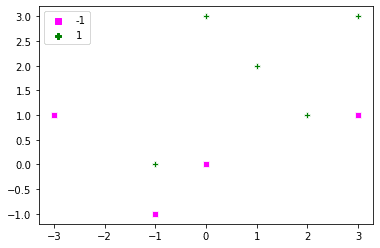
Let’s define a very simple dataset, the corresponding labels and a simple routine for plotting this data. Optionally, if a string of alphas is given to the plotting function, then it will also label all support vectors with their corresponding alpha values. Just to recall support vectors are those points for which $�>0$.

1 2 3 4 5 6 7 8 9 10 11 12 13 14 15 16

dat = np.array([[0, 3], [-1, 0], [1, 2], [2, 1], [3,3], [0, 0], [-1, -1], [-3, 1], [3, 1]]) labels = np.array([1, 1, 1, 1, 1, -1, -1, -1, -1])     def plot_x(x, t, alpha=[], C=0):     sns.scatterplot(dat[:,0], dat[:, 1], style=labels,     hue=labels, markers=['s', 'P'],     palette=['magenta', 'green'])     if len(alpha) > 0:         alpha_str = np.char.mod('%.1f', np.round(alpha, 1))         ind_sv = np.where(alpha > ZERO)[0]         for i in ind_sv:               plt.gca().text(dat[i,0], dat[i, 1]-.25, alpha_str[i] )                      plot_x(dat, labels)

The minimize() Function

Let’s look at the minimize() function in scipy.optimize library. It requires the following arguments:

• The objective function to minimize. Lagrange dual in our case.
• The initial values of variables with respect to which the minimization takes place. In this problem, we have to determine the Lagrange multipliers $�$. We’ll initialize all $�$ randomly.
• The method to use for optimization. We’ll use trust-constr.
• The linear constraints on $�$.
• The bounds on $�$.

Defining the Objective Function

Our objective function is ${�}_{�}$ defined above, which has to be maximized. As we are using the minimize() function, we have to multiply ${�}_{�}$ by (-1) to maximize it. Its implementation is given below. The first parameter for the objective function is the variable w.r.t. which the optimization takes place. We also need the training points and the corresponding labels as additional arguments.

You can shorten the code for the lagrange_dual() function given below by using matrices. However, in this tutorial, it is kept very simple to make everything clear.

1 2 3 4 5 6 7 8 9

# Objective function def lagrange_dual(alpha, x, t):     result = 0     ind_sv = np.where(alpha > ZERO)[0]     for i in ind_sv:         for k in ind_sv:             result = result + alpha[i]*alpha[k]*t[i]*t[k]*np.dot(x[i, :], x[k, :])     result = 0.5*result - sum(alpha)         return result

Defining the Linear Constraints

The linear constraint on alpha for each point is given by:

$$\sum _{�}{�}_{�}{�}_{�}=0$$

We can also write this as:
$${�}_0{�}_0+{�}_1{�}_1+\dots {�}_{�}{�}_{�}=0$$

The LinearConstraint() method requires all constraints to be written as matrix form, which is:

$$0=\left[\begin{array}{ccc}{�}_0& {�}_1& \dots {�}_{�}\end{array}\right]\left[\begin{array}{c}{�}_0\\ {�}_1\\ ⋮\\ {�}_{�}\end{array}\right]=0$$

The first matrix is the first parameter in the LinearConstraint() method. The left and right bounds are the second and third arguments.

1 2	linear_constraint = LinearConstraint(labels, [0], [0]) print(linear_constraint)

1	<scipy.optimize._constraints.LinearConstraint object at 0x12c87f5b0>

Defining the Bounds

The bounds on alpha are defined using the Bounds() method. All alphas are constrained to lie between 0 and $�$. Here is an example for $�=10$.

1 2	bounds_alpha = Bounds(np.zeros(dat.shape[0]), np.full(dat.shape[0], 10)) print(bounds_alpha)

1	Bounds(array([0., 0., 0., 0., 0., 0., 0., 0., 0.]), array([10, 10, 10, 10, 10, 10, 10, 10, 10]))

Defining the Function to Find Alphas

Let’s write the overall routine to find the optimal values of alpha when given the parameters x, t, and C. The objective function requires the additional arguments x and t, which are passed via args in minimize().

1 2 3 4 5 6 7 8 9 10 11 12 13 14 15 16

def optimize_alpha(x, t, C):     m, n = x.shape     np.random.seed(1)     # Initialize alphas to random values     alpha_0 = np.random.rand(m)*C     # Define the constraint     linear_constraint = LinearConstraint(t, [0], [0])     # Define the bounds     bounds_alpha = Bounds(np.zeros(m), np.full(m, C))     # Find the optimal value of alpha     result = minimize(lagrange_dual, alpha_0, args = (x, t), method='trust-constr',                       hess=BFGS(), constraints=[linear_constraint],                       bounds=bounds_alpha)     # The optimized value of alpha lies in result.x     alpha = result.x     return alpha

Determining the Hyperplane

The expression for the hyperplane is given by:
$${�}^{�}�+{�}_0=0$$

For the hyperplane, we need the weight vector $�$ and the constant ${�}_0$. The weight vector is given by:
$$�=\sum _{�}{�}_{�}{�}_{�}{�}_{�}$$

If there are too many training points, it’s best to use only support vectors with $�>0$ to compute the weight vector.

For ${�}_0$, we’ll compute it from each support vector $�$, for which ${�}_{�}<�$, and then take the average. For a single support vector ${�}_{�}$, ${�}_0$ is given by:

$${�}_0={�}_{�}–{�}^{�}{�}_{�}$$

A support vector’s alpha cannot be numerically exactly equal to C. Hence, we can subtract a small constant from C to find all support vectors with ${�}_{�}<�$. This is done in the get_w0() function.

1 2 3 4 5 6 7 8 9 10 11 12 13 14 15 16 17 18

def get_w(alpha, t, x):     m = len(x)     # Get all support vectors     w = np.zeros(x.shape[1])     for i in range(m):         w = w + alpha[i]*t[i]*x[i, :]             return w   def get_w0(alpha, t, x, w, C):     C_numeric = C-ZERO     # Indices of support vectors with alpha<C     ind_sv = np.where((alpha > ZERO)&(alpha < C_numeric))[0]     w0 = 0.0     for s in ind_sv:         w0 = w0 + t[s] - np.dot(x[s, :], w)     # Take the average         w0 = w0 / len(ind_sv)     return w0

Classifying Test Points

To classify a test point ${�}_{����}$, we use the sign of $�({�}_{����})$ as:

$${\text{label}}_{{�}_{����}}=\text{sign}(�({�}_{����}))=\text{sign}({�}^{�}{�}_{����}+{�}_0)$$

Let’s write the corresponding function that can take as argument an array of test points along with $�$ and ${�}_0$ and classify various points. We have also added a second function for calculating the misclassification rate:

1 2 3 4 5 6 7 8 9 10 11 12

def classify_points(x_test, w, w0):     # get y(x_test)     predicted_labels = np.sum(x_test*w, axis=1) + w0     predicted_labels = np.sign(predicted_labels)     # Assign a label arbitrarily a +1 if it is zero     predicted_labels[predicted_labels==0] = 1     return predicted_labels   def misclassification_rate(labels, predictions):     total = len(labels)     errors = sum(labels != predictions)     return errors/total*100

Plotting the Margin and Hyperplane

Let’s also define functions to plot the hyperplane and the soft margin.

1 2 3 4 5 6 7 8 9 10 11

def plot_hyperplane(w, w0):     x_coord = np.array(plt.gca().get_xlim())     y_coord = -w0/w[1] - w[0]/w[1] * x_coord     plt.plot(x_coord, y_coord, color='red')   def plot_margin(w, w0):     x_coord = np.array(plt.gca().get_xlim())     ypos_coord = 1/w[1] - w0/w[1] - w[0]/w[1] * x_coord     plt.plot(x_coord, ypos_coord, '--', color='green')     yneg_coord = -1/w[1] - w0/w[1] - w[0]/w[1] * x_coord     plt.plot(x_coord, yneg_coord, '--', color='magenta')

Powering Up The SVM

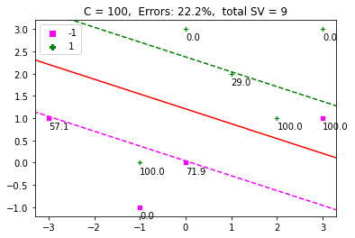
It’s now time to run the SVM. The function display_SVM_result() will help us visualize everything. We’ll initialize alpha to random values, define C and find the best values of alpha in this function. We’ll also plot the hyperplane, the margin and the data points. The support vectors would also be labelled by their corresponding alpha value. The title of the plot would be the percentage of errors and number of support vectors.

1 2 3 4 5 6 7 8 9 10 11 12 13 14 15 16 17 18 19 20 21 22

def display_SVM_result(x, t, C):     # Get the alphas     alpha = optimize_alpha(x, t, C)       # Get the weights     w = get_w(alpha, t, x)     w0 = get_w0(alpha, t, x, w, C)     plot_x(x, t, alpha, C)     xlim = plt.gca().get_xlim()     ylim = plt.gca().get_ylim()     plot_hyperplane(w, w0)     plot_margin(w, w0)     plt.xlim(xlim)     plt.ylim(ylim)     # Get the misclassification error and display it as title     predictions = classify_points(x, w, w0)     err = misclassification_rate(t, predictions)     title = 'C = ' + str(C) + ',  Errors: ' + '{:.1f}'.format(err) + '%'     title = title + ',  total SV = ' + str(len(alpha[alpha > ZERO]))     plt.title(title)      display_SVM_result(dat, labels, 100)     plt.show()

The Effect of C

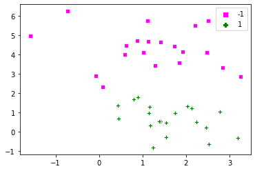
If you change the value of C to $\mathrm{\infty }$, then the soft margin turns into a hard margin, with no toleration for errors. The problem we defined above is not solvable in this case. Let’s generate an artificial set of points and look at the effect of C on classification. To understand the entire problem, we’ll use a simple dataset, where the positive and negative examples are separable.

Below are the points generated via make_blobs():

1 2 3 4 5

dat, labels = dt.make_blobs(n_samples=[20,20],                            cluster_std=1,                            random_state=0) labels[labels==0] = -1 plot_x(dat, labels)

Now let’s define different values of C and run the code.

1 2 3 4 5 6 7 8 9

fig = plt.figure(figsize=(8,25))   i=0 C_array = [1e-2, 100, 1e5]   for C in C_array:     fig.add_subplot(311+i)         display_SVM_result(dat, labels, C)       i = i + 1

Comments on the Result

The above is a nice example, which shows that increasing $�$, decreases the margin. A high value of $�$ adds a stricter penalty on errors. A smaller value allows a wider margin and more misclassification errors. Hence, $�$ defines a tradeoff between the maximization of margin and classification errors.

Consolidated Code

Here is the consolidated code, that you can paste in your Python file and run it at your end. You can experiment with different values of $�$ and try out the different optimization methods given as arguments to the minimize() function.

1 2 3 4 5 6 7 8 9 10 11 12 13 14 15 16 17 18 19 20 21 22 23 24 25 26 27 28 29 30 31 32 33 34 35 36 37 38 39 40 41 42 43 44 45 46 47 48 49 50 51 52 53 54 55 56 57 58 59 60 61 62 63 64 65 66 67 68 69 70 71 72 73 74 75 76 77 78 79 80 81 82 83 84 85 86 87 88 89 90 91 92 93 94 95 96 97 98 99 100 101 102 103 104 105 106 107 108 109 110 111 112 113 114 115 116 117 118 119 120 121 122 123 124 125 126 127 128 129 130 131 132 133 134 135

import numpy as np     # For optimization from scipy.optimize import Bounds, BFGS                     from scipy.optimize import LinearConstraint, minimize   # For plotting import matplotlib.pyplot as plt import seaborn as sns # For generating dataset import sklearn.datasets as dt   ZERO = 1e-7   def plot_x(x, t, alpha=[], C=0):     sns.scatterplot(dat[:,0], dat[:, 1], style=labels,     hue=labels, markers=['s', 'P'],     palette=['magenta', 'green'])     if len(alpha) > 0:         alpha_str = np.char.mod('%.1f', np.round(alpha, 1))         ind_sv = np.where(alpha > ZERO)[0]         for i in ind_sv:               plt.gca().text(dat[i,0], dat[i, 1]-.25, alpha_str[i] )   # Objective function def lagrange_dual(alpha, x, t):     result = 0     ind_sv = np.where(alpha > ZERO)[0]     for i in ind_sv:         for k in ind_sv:             result = result + alpha[i]*alpha[k]*t[i]*t[k]*np.dot(x[i, :], x[k, :])     result = 0.5*result - sum(alpha)         return result   def optimize_alpha(x, t, C):     m, n = x.shape     np.random.seed(1)     # Initialize alphas to random values     alpha_0 = np.random.rand(m)*C     # Define the constraint     linear_constraint = LinearConstraint(t, [0], [0])     # Define the bounds     bounds_alpha = Bounds(np.zeros(m), np.full(m, C))     # Find the optimal value of alpha     result = minimize(lagrange_dual, alpha_0, args = (x, t), method='trust-constr',                       hess=BFGS(), constraints=[linear_constraint],                       bounds=bounds_alpha)     # The optimized value of alpha lies in result.x     alpha = result.x     return alpha   def get_w(alpha, t, x):     m = len(x)     # Get all support vectors     w = np.zeros(x.shape[1])     for i in range(m):         w = w + alpha[i]*t[i]*x[i, :]             return w   def get_w0(alpha, t, x, w, C):     C_numeric = C-ZERO     # Indices of support vectors with alpha<C     ind_sv = np.where((alpha > ZERO)&(alpha < C_numeric))[0]     w0 = 0.0     for s in ind_sv:         w0 = w0 + t[s] - np.dot(x[s, :], w)     # Take the average         w0 = w0 / len(ind_sv)     return w0   def classify_points(x_test, w, w0):     # get y(x_test)     predicted_labels = np.sum(x_test*w, axis=1) + w0     predicted_labels = np.sign(predicted_labels)     # Assign a label arbitrarily a +1 if it is zero     predicted_labels[predicted_labels==0] = 1     return predicted_labels   def misclassification_rate(labels, predictions):     total = len(labels)     errors = sum(labels != predictions)     return errors/total*100   def plot_hyperplane(w, w0):     x_coord = np.array(plt.gca().get_xlim())     y_coord = -w0/w[1] - w[0]/w[1] * x_coord     plt.plot(x_coord, y_coord, color='red')   def plot_margin(w, w0):     x_coord = np.array(plt.gca().get_xlim())     ypos_coord = 1/w[1] - w0/w[1] - w[0]/w[1] * x_coord     plt.plot(x_coord, ypos_coord, '--', color='green')     yneg_coord = -1/w[1] - w0/w[1] - w[0]/w[1] * x_coord     plt.plot(x_coord, yneg_coord, '--', color='magenta')     def display_SVM_result(x, t, C):     # Get the alphas     alpha = optimize_alpha(x, t, C)       # Get the weights     w = get_w(alpha, t, x)     w0 = get_w0(alpha, t, x, w, C)     plot_x(x, t, alpha, C)     xlim = plt.gca().get_xlim()     ylim = plt.gca().get_ylim()     plot_hyperplane(w, w0)     plot_margin(w, w0)     plt.xlim(xlim)     plt.ylim(ylim)     # Get the misclassification error and display it as title     predictions = classify_points(x, w, w0)     err = misclassification_rate(t, predictions)     title = 'C = ' + str(C) + ',  Errors: ' + '{:.1f}'.format(err) + '%'     title = title + ',  total SV = ' + str(len(alpha[alpha > ZERO]))     plt.title(title)      dat = np.array([[0, 3], [-1, 0], [1, 2], [2, 1], [3,3], [0, 0], [-1, -1], [-3, 1], [3, 1]]) labels = np.array([1, 1, 1, 1, 1, -1, -1, -1, -1])                   plot_x(dat, labels) plt.show() display_SVM_result(dat, labels, 100)     plt.show()   dat, labels = dt.make_blobs(n_samples=[20,20],                            cluster_std=1,                            random_state=0) labels[labels==0] = -1 plot_x(dat, labels)   fig = plt.figure(figsize=(8,25))   i=0 C_array = [1e-2, 100, 1e5]   for C in C_array:     fig.add_subplot(311+i)         display_SVM_result(dat, labels, C)       i = i + 1

 

Further Reading

This section provides more resources on the topic if you are looking to go deeper.

Books

• Pattern Recognition and Machine Learning by Christopher M. Bishop

Articles

• Support Vector Machines for Machine Learning
• A Tutorial on Support Vector Machines for Pattern Recognition by Christopher J.C. Burges

API Reference

• SciPy’s optimization library
• Scikit-learn’s sample generation library (sklearn.datasets)
• NumPy random number generator

Summary

In this tutorial, you discovered how to implement an SVM classifier from scratch.

Specifically, you learned:

• How to write the objective function and constraints for the SVM optimization problem
• How to write code to determine the hyperplane from Lagrange multipliers
• The effect of C on determining the margin

Do you have any questions about SVMs discussed in this post? Ask your questions in the comments below and I will do my best to answer.